How the integration diagnostics work
When frames are stacked, three questions are worth asking of the result: where did the
combine throw samples away, how many frames and how much weight did each pixel get, and
how much quieter is the stack than one frame, against what the square root of the number of
frames promises. And one about the picture itself: what do the histograms of its channels
look like. valerian stack --science-report and valerian drizzle --science-report answer
them with maps, a curve and histograms, and valerian plot draws any of them on its own. The
desktop app has them in the Science panel of the Stack step. For a worked example start with
tutorial 14; this page says what each output is, how it is made
and what every option and control does.
The maps of a stack
The combine looks at each pixel's stack of values, one per frame, rejects outliers and takes the weighted mean of the rest (see How stacking works). With the maps on, it also records for every pixel:
| Map | File stem | What each pixel holds |
|---|---|---|
| Rejected low | rejection_low |
how many samples were thrown out for being below the centre of the pixel's values, summed over the colour planes |
| Rejected high | rejection_high |
how many were thrown out for being above it, summed over the colour planes |
| Pixel count | pixel_count |
how many samples went into the mean (the frames that had data, less those rejected), first plane |
| Weight | weight_map |
the summed weight of those samples, first plane. The weights are scaled to a mean of 1, so it is about the pixel count when the frames are alike and smaller where the heavy frames were rejected or missing |
"Centre" is the median of the values that survived the rejection, so a rejected sample is low or high according to which side of it the sample lies. Satellite trails, cosmic rays and hot pixels show as high rejections (a bright outlier); dark outliers, the shadow of a dust speck on one frame or a cold pixel, as low ones. A map that is flat noise is a healthy stack. Structure in it means something: a ridge along an edge is where the dither left few frames, a bright patch on the high map is a gradient or a bright region the frames do not agree on, and a bright dot is a star that moved or a satellite.
Each map is written as a PNG (reduced by block means to at most 1000 pixels on the long side,
with a colour bar from zero to the largest value and the minimum, median, mean, maximum and the
share of pixels that are zero), as a full-size 32-bit FITS file (.fits) and, for the
rejection and count maps, as a CSV of how many pixels hold each value (.csv). The rejection
maps need the CPU combiner: with --science-report the stack is made on the CPU even when a
graphics card is present, and says so.
The maps of a drizzle
valerian drizzle --science-report writes the three maps of the output grid (first plane),
with drizzle_ in front of their names:
| Map | File stem | What each output pixel holds |
|---|---|---|
| Weight | drizzle_weight_map |
the summed overlap area times frame weight of the drops that reached it; low values are thinly covered |
| Pixel count | drizzle_pixel_count |
how many input pixels (drops) reached it, saturating at 65535 |
| Rejected | drizzle_rejected |
how many input pixels the second pass rejected as outliers, counted at the output pixel their centre falls in; all zero with --no-reject |
A raw Bayer mosaic is dropped into its own colour planes, so the first plane's count is of red drops only.
Noise against the square root of the number of frames
For N equal frames of independent noise, the noise of their mean falls as 1/sqrt(N). The
noise curve measures how closely a real stack follows that, without a model of the noise:
- The registered frames (one plane each, the middle one for a colour image, on the reference grid, levels matched as the stack matches them) and their stack weights are taken. Only pixels where every frame has data are used, sampled to about 400 000.
- For each power of two
mup to half the frames (and the largestm, if the count is not a power of two), the first2mframes are split alternately into two sets. Each set's weighted mean is a stack ofmframes, with the same weights as the real stack but without the rejection. - The difference of the two means contains twice the variance of one: the noise of an
m-frame stack is the standard deviation of the difference over the square root of two. The standard deviation is clipped at 3 sigma (so a star the frames disagree on does not count) and divided by 0.9866, the standard deviation of a Gaussian truncated at 3 sigma. - The noise of one frame is the same measurement on up to eight disjoint pairs of single
frames, averaged. The expectation at
mframes is that value oversqrt(m).
This does not depend on how the noise is spread between neighbouring pixels, so it is not fooled
by the correlation that resampling puts between them (which would make an estimator based on
neighbouring pixels read low), and it is the noise the stack really has at those pixels. The
table has, for each m: the measured noise, the expectation, their ratio, the reduction
(one frame over measured) and sqrt(m). A ratio above 1 means the stack is noisier than
independent equal frames would be, because the frames are unequal (clouds raise some frames'
noise, and the weights cannot undo all of it), or because the noise is not entirely independent
between frames (a shared pattern would show as a curve that flattens). A curve that lies on the
line means the frames really are independent and alike.
The result is shown on a plot with both axes logarithmic (a straight line is a power law). It needs at least four registered frames.
Histograms
histogram.png shows one histogram per channel of the result, twice:
- Linear: 256 bins from the 0.01th to the 99.99th percentile of all channels, so they can be compared, on a logarithmic count axis (log10 of the pixels plus one). The sky is the tall peak; its width is the noise, and the long tail to the right is the stars and the target.
- Stretched: the same pixels after the automatic midtone stretch of the luminance (black point 2.8 robust sigmas below the sky, midtone solved to put the sky at 25 per cent), applied to every channel alike so the colour balance is what the picture would show. A channel whose peak sits left of the others has a lower sky; one whose peak is cut off at 0 has pixels at or below the black point.
histogram.csv holds the counts of both (view, bin_lo, bin_hi, one column per channel).
integration.json holds, per channel, the minimum, maximum, median, robust sigma, the fractions
of pixels clipped to 0 and to 1 by the stretch and the stretched median, and the stretch used
(black, white, midtone).
Files and options
--science-report <DIR> on valerian stack and valerian drizzle adds the section to a report
folder (with valerian stack it also holds the subframe analysis, and the
limit options of that page apply). It writes rejection_low and rejection_high (stack) or
drizzle_rejected (drizzle), pixel_count, weight_map, each as .png, .fits and (for
counts) .csv; noise.png and noise.csv (stack); histogram.png and histogram.csv;
integration.json (drizzle_integration.json for a drizzle); and the page report.html, which
gathers them.
valerian plot <kind> INPUT -o FILE.png draws one:
| Kind | Input | Writes beside the PNG |
|---|---|---|
rejection-low, rejection-high, weight-map, count-map |
frames (stacked on the CPU with the defaults) | .fits of the map, .csv of its value counts (not for the weight map) |
noise |
frames | .csv and .json of the curve |
histogram |
one FITS image | .csv and .json |
--threshold <SIGMA> (5) is the star detection threshold of the registration. For a different
rejection, weights or normalisation, use valerian stack ... --science-report, which takes all
the stack options.
The Science panel in the desktop app
Open the Stack step, choose the Science chip, give a folder of frames and press Stack for the maps. It registers and stacks on the CPU (with progress and Cancel), and the chips above the viewer then offer Rejected low, Rejected high, Pixel count, Weight, Noise and Histogram next to Subframes; the panel says how many frames were stacked and the noise reduction against the square root. This stack is for looking at: it is not written to a file and does not replace the Mean stack. The frames the Use for stacking button left out are left out here too.
Checked against astropy and numpy
scripts/compare_python_integration.py repeats the maps and the noise curve with different code
on the 60 IC 5070 frames, for a stack made with equal weights, no level matching and 3 sigma
clipping (valerian register, then valerian stack --normalisation none --weights equal
--rejection sigma --science-report), over a band of 300 rows (astropy 8.0.2, numpy 2.5):
| Quantity | Valerian | Reference |
|---|---|---|
| rejection low map, mean per pixel (3 planes) | 0.038 | 0.038: astropy.stats.sigma_clip (median centre, standard deviation about it, 10 iterations), identical in 100.00 % of the pixels |
| rejection high map, mean per pixel | 1.580 | 1.580, identical in 100.00 % of the pixels |
| pixel count map, mean | 57.451 | 57.451, identical in 100.00 % of the pixels |
| noise, 1 frame, ADU | 46.84 | 46.61: two means of the first 2m frames, sigma_clipped_stats of their difference over the square root of two |
| 2 frames per half | 33.40 | 33.10 |
| 4 | 23.39 | 23.24 |
| 8 | 16.15 | 15.97 |
| 16 | 11.91 | 11.54 |
| 30 | 8.79 | 8.26 |
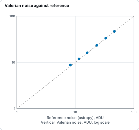
Noise of the mean of 2m frames, Valerian against the astropy reference on log axes, from the table above: the points drift above the dashed line at 16 and 30 frames.
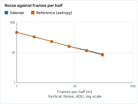
Noise of the mean of 2m frames, Valerian against the astropy reference, from the table above: they part by 6 per cent at 30 frames.
The maps are the same counts, pixel for pixel, as an independent clipping of the same registered frames. The noise curve agrees to 0.5 to 1.1 per cent up to 8 frames per half and reads 3 and 6 per cent higher at 16 and 30: Valerian measures the whole frame (about 400 000 sampled pixels) and the reference a band through the middle, and the larger the stack the more a gradient or a residual pattern in the outer parts counts against it, since the random noise has averaged down. The frames at the large end are also the ones with the clouds.
Limits of the method
- The noise curve measures the mean of the registered frames with the stack's weights, not the rejected stack. Rejection removes outliers without changing the noise of what is left much, but it does remove some samples, so the real stack is a little noisier than the curve suggests at pixels with many rejections.
- The count and weight maps are of the first colour plane; the rejection maps are summed over the planes, so a pixel can show up to three times as many rejections as frames.
- The histograms are of the pixels with data; the empty border of a stack (NaN) is left out.