Tutorial 14: Integration diagnostics¶

Goal: see what the combine did to your stack. Where did it throw samples away, how many frames and how much weight did each pixel get, how much quieter is the stack than a single frame against what the square root of the number of frames promises, and what do the histograms of the channels look like, before and after stretching. You finish with a folder of maps (PNG, FITS and CSV), a noise curve, histograms and a one-file HTML report, for a stack and for a drizzle.

Data: the sixty IC 5070 Seestar lights of tutorial 4, in lights/.

What happens. The stack is made on the CPU with the per-pixel books kept, and the noise is measured from split halves of the registered frames. How each output is made is in How the integration diagnostics work.

Step 1: Stack with the report¶

valerian stack lights/ -o stack.fits --science-report integration

read 60 frames in 123.1ms
compute: CPU (the rejection maps and the noise curve need the CPU combiner)
reference candidate frame 47: 59 of 59 other frames register
reference: frame 47 (FWHM 2.16 px)
combining 60 frames with LinearFit { low: 5.0, high: 2.5 }, weights NoiseFwhm
...
60 of 60 frames stacked with LinearFit { low: 5.0, high: 2.5 }, reference frame 47 (Light_IC 5070_10.0s_LP_20260728-224223.fit), 15.5s
wrote stack.fits
wrote integration/subframes.csv
...
wrote integration/rejection_low.png
wrote integration/rejection_low.fits
wrote integration/rejection_low.csv
wrote integration/rejection_high.png
...
wrote integration/weight_map.fits
wrote integration/histogram.png
wrote integration/histogram.csv
wrote integration/noise.png
wrote integration/noise.csv
wrote integration/integration.json
wrote integration/report.html

It took 15.5 s on the 24-core server (the graphics-card stack of tutorial 4 took 12.2 s; the maps need the CPU combiner, so --backend has no effect here). The report folder also holds the subframe analysis of the same frames, on the same report.html.

Step 2: Where were samples thrown away¶

Open integration/rejection_high.png.

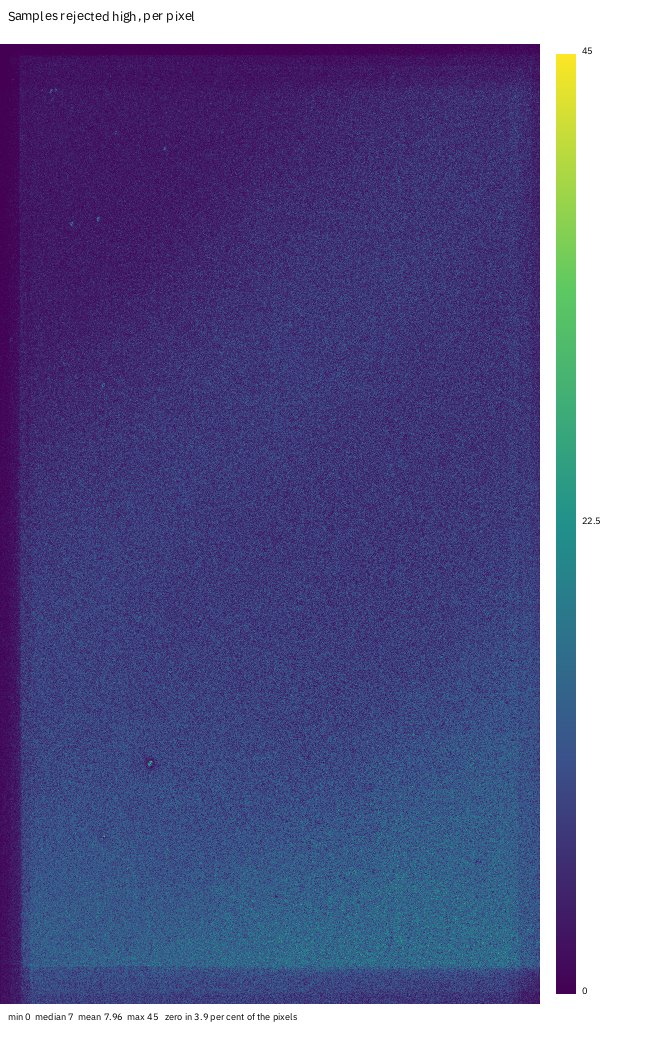
Every pixel is a stack of 60 samples; each map pixel is how many of them the linear-fit clipping threw out for being above the centre (summed over red, green and blue, so the three planes can add up to more than 60). The colour bar runs from 0 to 45; the median is 7 and the mean 7.96 per pixel, and 3.9 per cent of the pixels lost none. The rejection is a salt of noise, as it should be for a stack with a rejection limit of 2.5 sigma on the high side. Three things are not noise:

• the dark stripe along the left edge and the lighter band along the top and bottom: few frames cover those pixels, so there is little to reject;
• the brighter band along the bottom: the sky is brighter there (a gradient), the frames disagree more about it and the high-side clipping removes more;
• a few bright dots: stars or defects the frames disagree on (a variable star, a hot pixel that moved with the dither, a satellite).

The low side is gentler (limit 5 sigma):

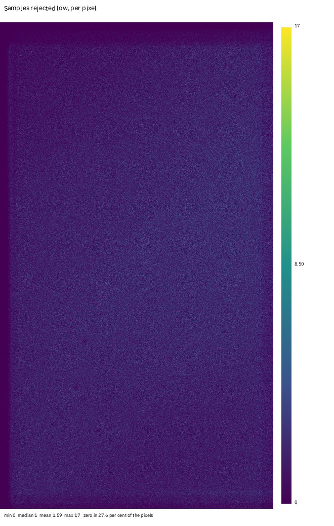
Mean 1.59 samples per pixel, at most 17, and 27.6 per cent of the pixels lost none. The maps have a CSV each (rejection_high.csv) with how many pixels have each count, so you can read the distribution: for the high map it peaks at 5 rejections (7.9 per cent of the pixels) and is Poisson-like around it.

If a map showed a bright streak, a satellite trail that crossed some frames, you would see it here as a line of rejections along its path; if it showed a bright ring, a dust shadow that moved between frames. A map with a hot region over the target means the frames disagree about the target itself (guiding trouble, or a change of focus), and the rejection is eating real signal.

Step 3: How many frames, how much weight¶

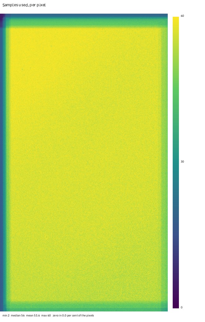
The pixel count map is the samples used per pixel: the frames that had data minus the ones rejected. Minimum 2 (a corner covered by two frames), median 56, mean 53.6, maximum 60, and no pixel without data. The pattern at the edges is the dither: the sixty frames are shifted by up to 100 pixels, and the border of the stack, a hundred pixels at most, has fewer frames. This is where the stack is noisier and where to crop.

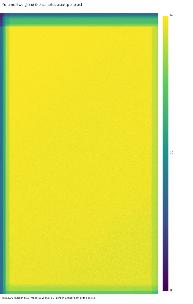
The weight map is the sum of the weights of the samples used. The weights have a mean of 1 across the frames, so it is near the count where the frames are alike (median 59.03, maximum 60, minimum 3.90). Where it is low while the count is high, the heavy frames were the ones rejected or missing, so the pixel is made of the poorer frames: that is the map to crop by.

Step 4: How much quieter than the square root¶

integration/noise.csv:

frames_per_half,noise_adu,sqrt_n_expectation_adu,measured_over_expected,reduction,sqrt_n
1,45.001,46.522,0.9673,1.034,1.000
2,34.877,32.896,1.0602,1.334,1.414
4,24.351,23.261,1.0468,1.911,2.000
8,16.405,16.448,0.9974,2.836,2.828
16,13.139,11.630,1.1297,3.541,4.000
30,9.439,8.494,1.1114,4.928,5.477

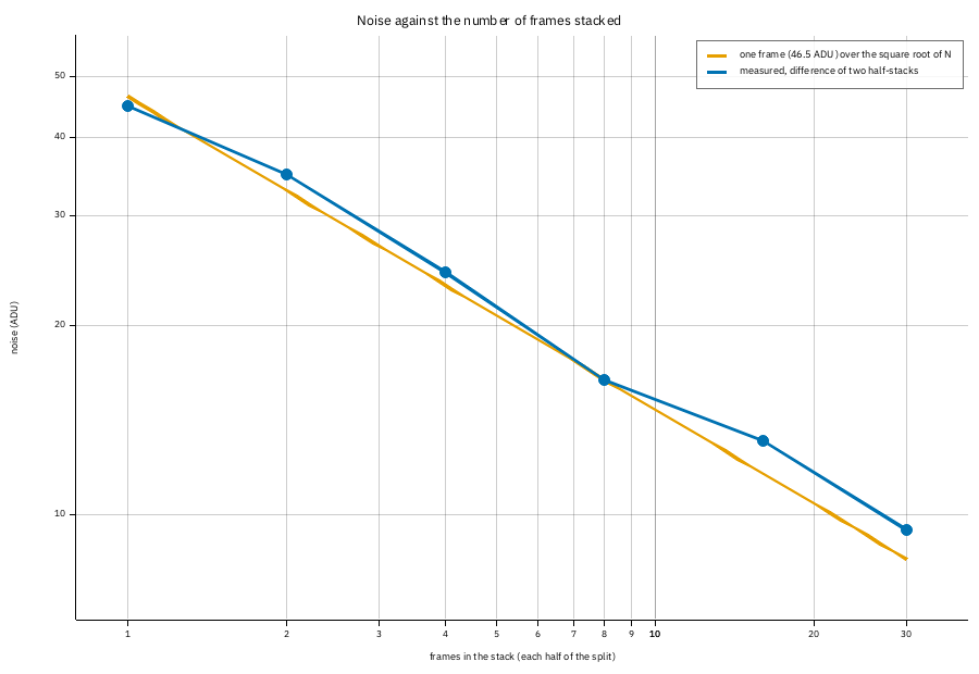
One frame has 46.5 ADU of noise (in the middle plane, the green). The blue line is the noise of a mean of 1, 2, 4, 8, 16 and 30 frames; the orange line is 46.5 over the square root of the number of frames. Up to 8 frames the measurement sits on the line (ratio 0.97 to 1.06; at 8 it is 0.997), as independent equal frames should. Past 8 it drifts above: at 30 frames the stack has 9.44 ADU against the 8.49 the law promises, a reduction of 4.93 against 5.48, 90 per cent of the theoretical. The frames are not equal: the cloud frames (23 to 30, 40, 41, 51, 52) have 10 to 40 per cent more noise than the good ones (47 to 55 ADU against 61 to 69), and the weights cannot make up for all of it. The frames come in time order, so the first 8 are the good ones and the later halves hold the cloud. That is the lesson of the curve: the square-root law is an upper limit that only frames of one quality reach. Leaving out the poor frames (tutorial 12) moves the curve closer to the line, at the price of fewer frames.

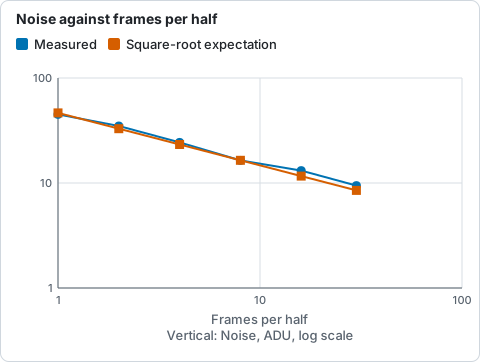
Measured noise of the mean of 1 to 30 frames against the square-root expectation, from the integration/noise.csv listing: the curve drifts above the line past 8 frames.

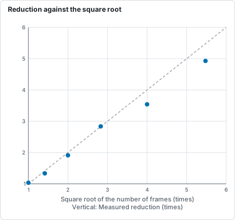
Noise reduction of the stack against the square root of the number of frames, from the noise.csv listing: the dashed line is the law, and the points leave it past 8 frames.

(The measurement is on the weighted mean of the registered frames without rejection, in the green plane. It is not the noise of stack.fits; it is how a stack of that many of these frames behaves.)

Step 5: The histograms¶

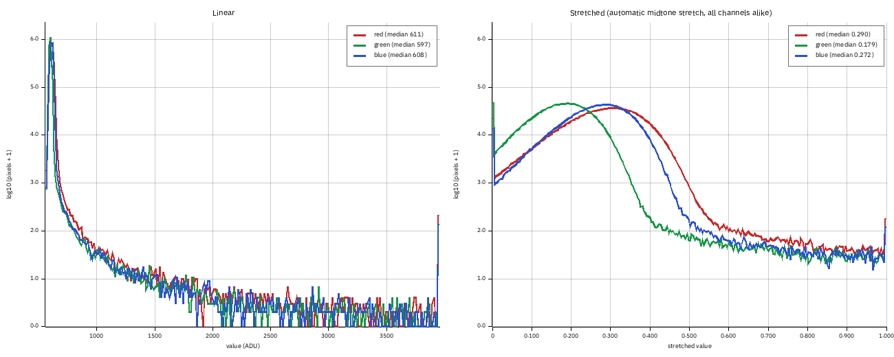
On the left, the linear histograms (256 bins from the 0.01th to the 99.99th percentile, 555 to 3957 ADU, on a logarithmic count axis): the sky is the tall peak at about 600 ADU in all three channels, and its width is the noise (robust sigma 12.6 red, 7.6 green, 10.2 blue). The long tail to the right is the stars and the nebula. On the right, the same after the automatic midtone stretch (black point 581.8 ADU, white point 5635.9, midtone balance 0.0139) applied to all three alike: the sky medians are 0.29 red, 0.18 green and 0.27 blue, which is the colour cast of the linear stack (the green sky sits lower than the red and the blue) made visible; a neutral stack would have the three peaks on top of one another. integration.json gives the fractions clipped: 1.03 per cent of the red pixels and 2.10 per cent of the green are at or below the black point, 0.006 per cent at or above the white point. The next tutorials fix the colour cast (tutorial 9).

Step 6: The same for a drizzle¶

valerian drizzle lights/ -o drizzle.fits --science-report integration-drizzle

It took 11.8 s and writes drizzle_weight_map, drizzle_pixel_count, drizzle_rejected (PNG and FITS, with a CSV of the counts for the last two), drizzle_histogram and drizzle_integration.json (2160 by 3840, scale 2, pixfrac 0.6).

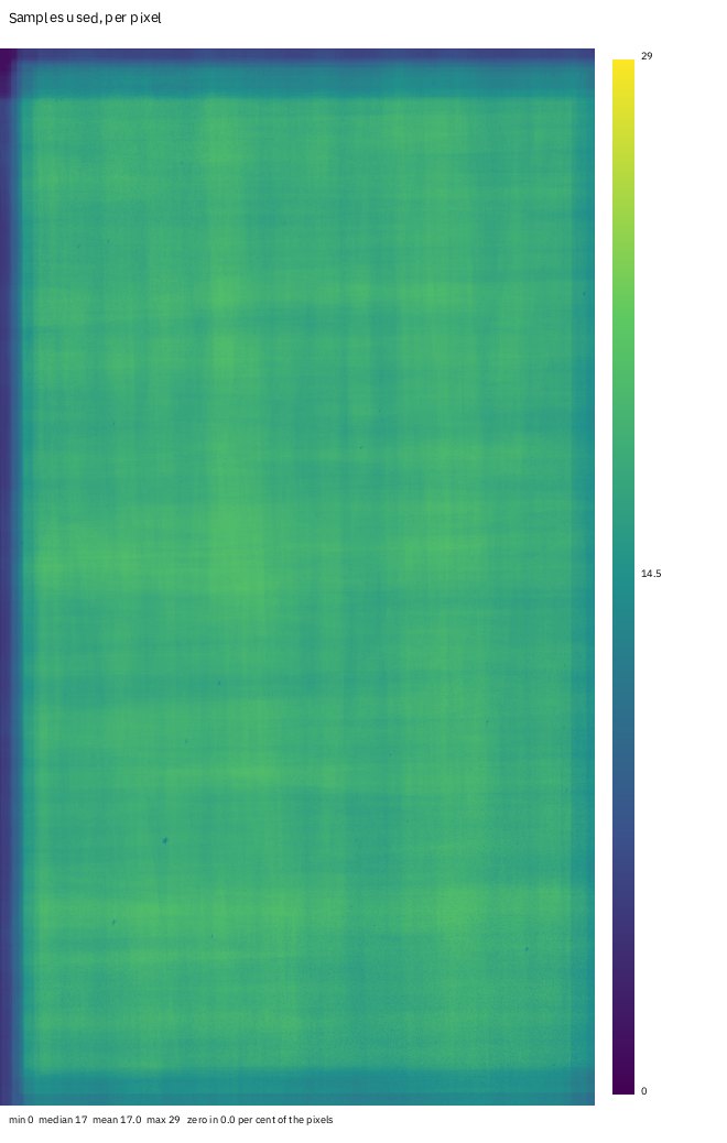
The pixel count is the number of input pixels that reached each output pixel: median 17, at most 29, mean 17.0, and 0.015 per cent of the output has none (holes). A drizzle of a raw Seestar mosaic drops each pixel into its own colour plane, so this is the count of red drops. The weight map (median 5.19, maximum 11.36) is the overlap area times the frame weight, and shows the same dither pattern. The rejected map is the second pass, which throws out input pixels more than 4 sigma from the first result: mean 0.0335 per output pixel, at most 5, and 96.8 per cent of the pixels lost none.

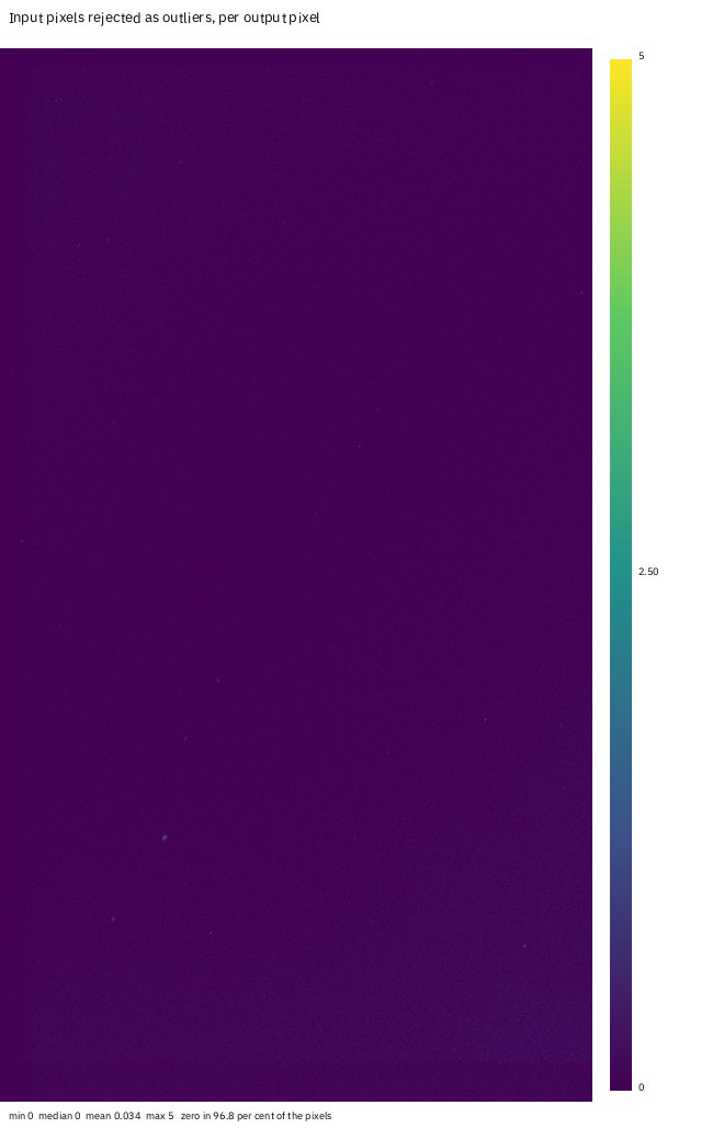
Holes are the reason to look at the count: a drizzle with too small a pixfrac or too few frames has output pixels no drop reached, which appear as black in the weight and count maps and as NaN in the image. See tutorial 10.

Step 7: One output at a time¶

valerian plot rejection-high lights/ -o rejected-high.png
valerian plot count-map lights/ -o count.png
valerian plot weight-map lights/ -o weight.png
valerian plot noise lights/ -o noise.png
valerian plot histogram stack.fits -o histogram.png

The four that need frames stack them on the CPU with the default settings; each writes the PNG and its data beside it (the map as .fits, the counts and the curve as .csv). valerian plot histogram reads any FITS image: a stack, a stretched picture, a single frame, and prints the median, sigma and clipped fractions of each channel:

red    median 610.8  sigma 12.64  black-clipped 1.031 %  white-clipped 0.006 %
green  median 597.3  sigma 7.55  black-clipped 2.103 %  white-clipped 0.004 %
blue   median 608.4  sigma 10.22  black-clipped 0.618 %  white-clipped 0.004 %

For the maps of a stack made with other settings (a different rejection or weights), use valerian stack ... --science-report, which takes all the stack options.

Step 8: The same in the desktop app¶

Open the Stack step, choose the Science chip, give the folder of frames and press Stack for the maps. It stacks on the CPU with progress and Cancel; then Rejected low, Rejected high, Pixel count, Weight, Noise and Histogram appear above the viewer next to Subframes.

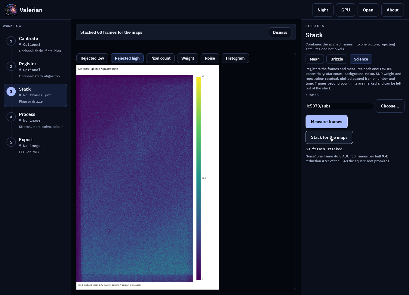
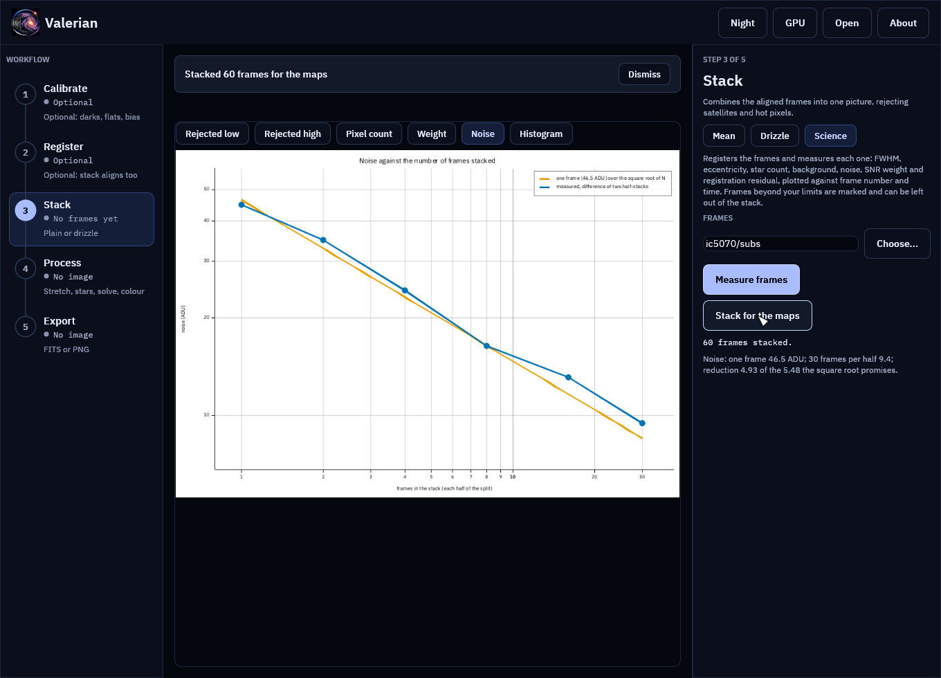
This stack is for looking at: it is not saved, and it does not replace the Mean stack. Every control is in the desktop app reference.

Options used¶

All options are in the command line reference.

How to tell it worked¶

• The report folder holds the maps, noise.png, histogram.png, integration.json and report.html.
• pixel_count.fits has a maximum equal to the number of frames and a minimum of the frames that cover the corner; its median is a little under the number of frames (the rejections).
• The noise table's first row has a reduction of 1.0 and the last has a reduction close to the square root of its frames (90 per cent here).
• The histograms have one tall sky peak per channel.

Troubleshooting¶

the noise curve needs at least 4 registered frames. Fewer than four frames registered, so there are no halves to compare. Stack more frames.

The maps are all zero. The rejection was off (--rejection none) or --rejection minmax with nothing to reject at that depth. The count map is still there.

The noise stays above the line. The frames are unequal (clouds, a changing sky: see the subframe analysis) or not independent (the same hot pixels or pattern noise in every frame, which averaging cannot remove: calibrate the frames, tutorial 2). A curve that flattens as frames are added means a shared pattern.

The histogram of one channel is cut off at the left. Pixels are at or below the black point of the stretch; integration.json gives the fraction. Run the background extraction and colour calibration (tutorials 5 and 9) before judging the balance.

It takes longer than the stack alone. The maps and the noise curve are made on the CPU. Make the stack on the graphics card first (valerian stack), and the diagnostics only when you need them.